 HOME
HOME
 POSTS
POSTS
Initially, I was going to clean up my solution, dockerize it and share a repo on GitHub, but I’ve never really gotten around to doing it, so I decided at least to share a writeup here. This competition was somewhat special for me, since it was the first one I’ve been participating in seriously, so it’s more of a novice’s impression, rather than a veteran’s breakdown of things :)
First impression
The goal of the TGS Salt Identification Challenge was segmenting salt deposits in seismic images. The data consisted of 101x101 images along with corresponding depth values in feet, and it was accompanied by a brief explanation of the image capturing process and the physics involved.
Below are some samples from training set (examples of non-empty, empty, almost empty and “fancy” masks):
| id | depth | image | mask |
|---|---|---|---|
| 8ebceef687 | 321 | 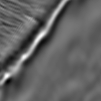 |
 |
| 0a7e067255 | 477 |  |
 |
| 00a3af90ab | 531 | 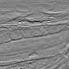 |
 |
| 8daf098aa9 | 594 | 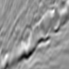 |
 |
At the start of the competition, it looked like a straightforward segmentation problem, perhaps with some smart way to incorporate depth information. Participants were more focused on technical questions, like:
What’s the optimal way of adapting the image size to a more conventional one?
UNet-like architectures, typically used for segmentation, require input dimensions to be divisible by 2 to the power of the number of downsampling layers. This is needed to ensure that “backward” path, that performs upscaling, ends up with the same set of resolutions to allow merging layer outputs from “parallel” paths.
Typical answers were resizing to 128 or 256 pixels or padding to 128 pixels, but what padding mode to use then? Participants have experimented with BORDER_REPLICATE and BORDER_REFLECT (in OpenCV terminology) and their different combinations (like mirror horizontally and repeat vertically), justifying this by physical nature of the data. After the competition deadline one team has shared another interesting approach, which they claim performed better in their setup: biharmonic inpainting, see [Argus] 14th place solution with full PyTorch pipeline for more details.
What are the best augmentations here?
Some participants argued that some “typical” ones, like random rotation, might be destroying important information (top/bottom arrangement). For me, the data was exotic enough to proceed entirely empirically :)
What loss function to use?
There were several approaches here, namely the “Kaggle forum approach” (Lovász loss + optionally BCE loss) and the “opendatascience community approach” (dice loss + BCE loss) with different weights. It seems that “ODS approach” was motivated by the successful experience of using such combination in previous segmentation-focused competition, and “Kaggle approach” was inspired by excited reports of using Lovász loss, which was advertised as a more direct way of optimizing Jaccard index. There was a bit of controversy around it, but experimentally it worked for several people, so it was still worth checking out. It was slightly trickier to use, which resulted in different variations by different participants: replacing ReLU with ELU+1 for better optimization (smoother), initially training with something common, like BCE, and then switching to Lovász, and most interesting one - using the symmetric version of Lovász loss.
What network capacity yields the best result on the provided data?
This was really interesting because during the competition several participants were reporting good results with ResNet-34 (which is considered to be small by modern standards), but after the end of the competition it turned out that many of the top entries included significantly bigger backbones, like SENet-154.
Last point was quite indicative of my overall impression from the competition - there was a lot of information on the dedicated Kaggle forum, but many of the described things seemed to work only in combination with something else, and of course asking for an ablation study would be too much, given limited time to research all the possible options :) Besides, as always, the devil is in the details, and getting all the things right simultaneously (architecture, optimizer, LR schedule, ensembling scheme) was more important than finding some “silver bullet” (relatively “tight” private leaderboard seems to confirm that)
Following best practices isn’t enough
After some time was spent on doing the “typical” research it turned out that result is still not there in terms of accuracy (compared to top entries in the leaderboard), so there was something that could be done to improve it, perhaps something competition-specific.
After looking closely at the metric (mean average precision), the main hypothesis was that almost empty masks were most problematic - they have only few positive pixels, so making a few-pixel misaligned prediction might “ruin” the whole sample. Another potential issue: if a model will try to “guess” such samples without having enough information (or capacity) to do this reliably - it might end up increasing the number of false positives, which are penalized in the same way (the sample gets a 0 score).
Surprisingly, the error analysis didn’t seem to confirm this - samples with different mask coverages seemed to contribute more or less equivalently to the overall error. Anyway, it seemed that treating samples with different mask coverage was beneficial, so I’ve tried different approaches to stratification. At first, I’ve made a mistake of simply binning all the samples according to “classes” of mask coverage (from empty to fully covered). Even though it seems right, in reality, it almost always mixes empty with almost empty masks, which goes directly against the purpose of such binning (unless you define the bins with the right limits explicitly). But even after fixing this, I didn’t observe improvement. When making this, I could’ve noticed the fact, that there are NO masks with 100% coverage, even though there are a lot of masks with 0% coverage. It turned out to be an important fact later on.
Approximately at this time, a lot of discussions related to deep supervision started to appear on the Kaggle forum. I wasn’t familiar with this concept, but it seemed like a neat idea, so I’ve decided to give it a try. The high-level idea is to introduce an additional training signal, which is supposed to help to learn features, which will be useful for the primary task. I’ve implemented something similar to this and have been finally observing some improvement. I tried slight variations, such as performing regression of mask coverage instead of classification, or multi-class classification (empty, almost empty, vertical, etc), but haven’t been able to get better results.
After implementing this and a few other tricks in decoder I felt that my experiments were stagnating, and it was time to experiment with heavier encoders. I’ve been running most of the experiments with ResNet34 encoder pretrained on ImageNet, as it was small enough to allow performing several experiments in parallel faster, than if I was doing the same thing with a bigger model. Unfortunately, I couldn’t just swap the encoder and retrain the model, many things needed to be adapted as well: decoder, batch size, LR schedule, etc. This (among other things) was preventing me from trying a wide variety of available encoders, and I ended up trying 3-4 most promising ones, and settling up on SE ResNeXt-50, which seemed to have the best “complexity”/”accuracy on ImageNet” trade-off. It resulted in a ~2x increase in training time per epoch, but the speed of convergence was comparable to my previous setup, and it eventually was outperforming it in terms of competition metric.
Team Merger deadline was getting closer and even though originally I was going to participate solo until the end to make it a learning experience, I started to doubt that it is the best strategy. Solo participants at the top of the leaderboard were started to be moved by larger teams, and not merging with someone else started to look sub-optimal. Of course, even a single participant might use a diverse ensemble to get “safer” predictions, but with multiple people in the team diversity is introduced into the ensemble more naturally, besides the amount of available hardware will increase as well. Finally, it doesn’t seem to contradict learning during the competition as long as the knowledge level among the teammates is comparable. Keeping this in mind, I decided to team up with Ivan Sosin, who was close to me on the public leaderboard. Merge went really well, and since we had quite different pipelines - there was a clear synergy between our models. Below is a high-level overview of my pipeline, and Ivan’s can be found here
Pipeline
Model: UNet-like architecture
Backbone: SE ResNeXt-50, pretrained on ImageNet
Decoder:
- Spatial and Channel Squeeze Excitation gating
- Hypercolumns
- Deep supervision (zero/nonzero mask)
Tile size adaptation:
- Pad 101 → 128
- Mode - replicate (reflect was worse, reflect horizontally+replicate vertically was same, random selection as an augmentation didn’t improve as well, although more tests needed to be made)
Augmentations:
- Random invert (unexpected, but visually it doesn’t change input dramatically. Also tried mean subtraction and derivative instead of raw input, but these didn’t work well)
- Random cutout (some papers indicate that it’s helpful for segmentation because implicitly it causes a model to learn “inpainting” input tiles)
- Random gamma-correction (makes sense, since tiles seem to be post-processed in a way that changes brightness)
- Random fixed-size crop
- Random horizontal flip
Optimizer:
- SGD: momentum 0.9, weight decay 0.0001
- Batch size: 16
- Starting LR determined using a procedure similar to LR find from fast.ai course - 5e-2
- LR schedule - cosine annealing from maximum LR, cycle length - 50 epochs, 10 cycles per experiment
- Best snapshots according to metric were saved independently for each cycle, the final solution uses 2 best cycles per fold
Loss:
- Since I used deep supervision it’s a combination of 3 losses - classification loss, pure segmentation loss (using the output from an earlier layer, empty samples excluded), total loss (segmentation loss over all samples)
- Classification loss - BCE
- Segmentation losses - BCE + Lavasz Hinge*0.5
- Segmentation loss was evaluated after cropping masks and predictions back to 101 - this seems to “fix” cases where a few-pixel corner mask was predicted on a padded mask with imperfect alignment but was cropped afterward, resulting in 0 metric per sample.
Cross-validation
- 5-fold random split
- Tried depth, area and “type”-based stratification, but it seemed to degrade the result
- Didn’t have enough time to synchronize folds with Ivan to allow cross-validation of ensemble results
Ensembling
Each of us trained multiple models (5 folds x 2 best cycles), which were used to predict masks. These 10 predictions were averaged per fold, and then a threshold was applied. Ivan chose a more conservative value of 0.5 for each fold, I selected a threshold that was resulting in the best metric - even though it might lead to overfitting to the validation set. Then ranges were aligned and predictions were averaged again; resulting predictions were thresholded and used for submission.
Post-processing
Few days before competition deadline we’ve decided to arrange predictions according to publicly shared CSV for mosaics. This was the “eureka” moment of the competition - ground truth annotation immediately became clear, and we started to look for ways to “help” the network solve the task better, taking the annotation specifics into account.
Unlike some other teams, we think that ground truth annotation made sense. It seems that the way the data was acquired makes it hard to get reasonable measurements underneath the salt domes, and also it seems that salt only forms a cap and doesn’t take the whole volume under this cap (I hope that people with domain expertise will correct if that’s a wrong assumption). In this case, it wasn’t physically-sound to label block underneath salt as salt (because probably they were not). Next question is why to label the salt dome thickness this particular way? Our hypothesis is that it’s hard to make this prediction given tiles without boundary, so they were marked as “not containing salt”, and the rest of the tiles were marked properly. Probably the tile size was chosen to match the expected thickness of the salt dome, but it’s just a guess.
Surprisingly, it turned out that our networks were already doing a very reasonable job in most cases and were just lacking enough context - a “bird’s eye view” should’ve been able to fix that. 2 days before the deadline we realized a way to do this - pass the tile ids along the pipeline and then apply post-processing heuristics using tile neighbor information to improve consistency of result, even though it was a bit risky (different depth values for neighboring samples probably imply that tiles were taken from different “slices” of a scan volume, so not necessarily they had aligned ground truth values).
We have used both ground truth and predicted masks to construct a few rules to improve the segmentation results:
- For almost-vertical ground truth tiles (the ones with last 30 rows same, but not fully covered) - extrapolate the last row downwards till the end of the mosaic
- For “caps” in ground truth tiles (the ones with fully-covered last row) - zero all tiles below
- For tiles vertically “sandwiched” between predicted or ground truth masks - replace mask with the last row of tile above, if it will cause increase of mask area (ideally it should’ve been a trapezoid from the last row of tile above to the first row of tile below, but didn’t have time to do that, and potential score gain is small)
- For tiles below predicted “caps” - do the same as for ground truth case
- For tiles below almost-vertical predicted tiles - extract downward.
Results
| model | local metric (single-fold) | public LB metric (5-fold ensemble) | private LB metric (5-fold ensemble) |
|---|---|---|---|
| Ivan’s best model | 0.859 | 0.866 | 0.881 |
| Mine best model | 0.865 | 0.872 | 0.887 |
| Team’s ensemble (TE) | - | 0.873 | 0.890 |
| TE + postprocessing | - | 0.881 | 0.892 |
It is interesting that although postprocessing heuristics improved public lb score significantly, the effect on private lb score was negligible (~0.1 increase vs 0.001). Some rules didn’t make a difference on public lb but deteriorated result on private lb significantly (last described rule caused 0.003 drop on private lb).
Another observation - seems that for the majority of teams private lb score is higher than the public nonetheless. It leads us to hypothesize that public/private split wasn’t random and was cherry-picked to meet organizers’ demands in a better way. One hypothesis for why private lb score was usually higher than public - organizers excluded few-pixel masks (which were hard to predict, incurred a high penalty and probably weren’t important from a business standpoint) from the private set.
We didn’t experience significant shake-up and ended up finishing with 11th place and a gold medal, which is a great result, considering that at the beginning of competition my goal was to get any medal. On the other hand, it sets the bar quite high for the next competition I’ll decide to participate in :)
I was storing all my submissions locally, and after the competition ended I decided that they are no longer needed. But, on second thought - maybe we can make some cool and insightful visualizations from them? :)
I settled on the following scheme:
- order all submits chronologically
- keep only the ones that improve private lb metric
- assemble them in mosaics and use as frames of an animation
It would’ve been cooler if I had raw predictions - this would’ve allowed to also see the evolution of uncertainty in particular cases, but unfortunately, all I have is binary predictions, extracted from submission CSVs.
I expected to see model’s predictions be noisy at first and then converge to some reasonable solution. The result doesn’t really match this expectation but is still worth sharing I guess.
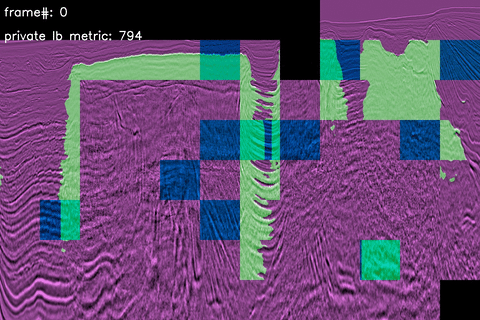
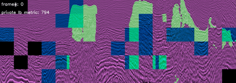
You can see which types of tiles are easy for the model and are predicted properly from the very first submits, and which are tricky even in the end (until they are replaced by mosaic-specific heuristics.
Few ones I found interesting in particular (blueish tiles are ground truth):
Mosaic 181
Mosaic 40
Mosaic 76

Mosaic 163
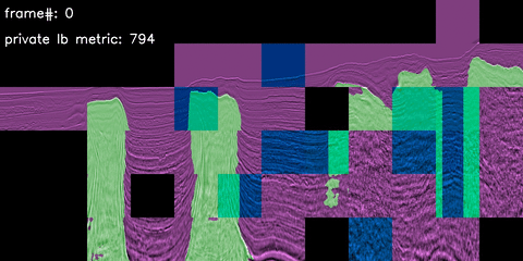
Judging from these animations, internal tiles annotated as empty ones aren’t difficult to classify - most are correctly predicted from the very first submission, which is scoring only 0.794 on private lb and doesn’t have any deep supervision.
Instead, vertical tiles on the boundary seem to be the trickiest, and some of them aren’t handled by the model even in the last submit. It leads to the hypothesis that provided crops don’t contain enough contextual information to reliably handle salt dome boundaries, which was among the main challenges of the competition.
Twitter Facebook Google+